A worked spatial example
The example below demonstrates how different spatial questions produce different priorities. Four fictional settlements share a transport network around a proposed project. Expected additional residents, water capacity, and seasonal clinic access are examined separately.
All locations and values are synthetic. They do not describe a real investment or community. The example is a teaching tool, not an empirical forecast, an engineering assessment, or a validated risk model. Coordinates are a local schematic grid in kilometres, without a geographic coordinate reference system.
The planning question
Suppose a project assessment identifies four plausible receiving settlements. The client needs to decide where to verify service conditions, which accommodation alternatives to examine, and what to discuss with public authorities before mobilisation.
A population-only ranking would prioritise Junction. A proportional water-shortfall ranking would prioritise Riverside. A wet-season access test would draw attention to Hill and Riverside. Each finding answers a different question.
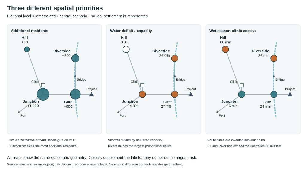
Figure 1. The same fictional geometry viewed through three planning questions. Counts, percentages, and minutes are labelled directly. The connecting lines show a schematic network, rather than a surveyed road alignment.
Define the assumptions
The initial population is 7,000 across four settlements. A single planning period adds 6% background growth without the project. Additional residents in the central scenario total 1,900; lower and higher scenarios use 950 and 2,850. These are assumed net additional residents present during that period, rather than cumulative gross arrivals.
The water calculation uses 40 litres per person per day solely to demonstrate arithmetic. It is not a recommendation for water-system design or a statement of adequate household provision. Real demand analysis needs applicable standards, service levels, losses, seasonal availability, quality, non-household uses, and differentiated demand.
For simplicity, each settlement has a separate reliable delivered water capacity and there is no transfer between systems. No additional commercial water demand is included. The example does not estimate storage, hydraulic constraints, or costs.
| Settlement | Initial population | Population without project | Additional residents: lower / central / higher | Delivered water capacity, L/day |
|---|---|---|---|---|
| Gate | 1,000 | 1,060 | 300 / 600 / 900 | 52,000 |
| Junction | 4,000 | 4,240 | 500 / 1,000 / 1,500 | 200,000 |
| Riverside | 800 | 848 | 120 / 240 / 360 | 32,000 |
| Hill | 1,200 | 1,272 | 30 / 60 / 90 | 60,000 |
The assumptions are in synthetic-example.json. A real application would attach a source and confidence assessment to every input, and separate observed capacity from planned upgrades.
Calculate demand and local deficits
For each settlement, multiply the population with the project by the assumed daily demand and subtract delivered capacity. Negative deficits become zero. Calculate the same quantity without the project to identify existing or background shortages.
For Gate in the central scenario:
| Settlement | Central population | Central demand, L/day | Deficit without project, L/day | Central deficit, L/day | Increase in deficit, L/day | Deficit / capacity |
|---|---|---|---|---|---|---|
| Gate | 1,660 | 66,400 | 0 | 14,400 | 14,400 | 27.7% |
| Junction | 5,240 | 209,600 | 0 | 9,600 | 9,600 | 4.8% |
| Riverside | 1,088 | 43,520 | 1,920 | 11,520 | 9,600 | 36.0% |
| Hill | 1,332 | 53,280 | 0 | 0 | 0 | 0.0% |
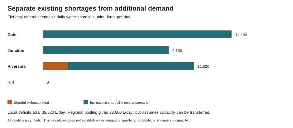
Figure 2. Riverside already has a deficit under background growth. The scenario increases that shortfall by 9,600 L/day. Separating these components supports a clearer conversation about contribution and cost-sharing.
Gate has the largest absolute deficit, while Riverside has the largest deficit relative to delivered capacity. Either measure can inform a decision, but neither establishes health consequences or a sufficient mitigation measure. Household access, quality, affordability, and service reliability still need investigation.
See what aggregation conceals
Central demand totals 372,800 L/day and capacity totals 344,000 L/day. Subtracting regional totals gives a shortfall of 28,800 L/day. Adding the deficits of the separate systems gives 35,520 L/day.
The difference is Hill's unused 6,720 L/day, which cannot simply be reassigned in the model. Regional pooling assumes a transfer that the network and operations may not permit. A real project needs to establish whether such transfer is feasible, reliable, affordable, and environmentally acceptable.
The same issue arises with clinic staffing, school places, wastewater treatment, and rental stock. An aggregate surplus does not establish that affected people can access it.
Compare scenarios without calling them probabilities
| Settlement | Lower deficit, L/day | Central deficit, L/day | Higher deficit, L/day |
|---|---|---|---|
| Gate | 2,400 | 14,400 | 26,400 |
| Junction | 0 | 9,600 | 29,600 |
| Riverside | 6,720 | 11,520 | 16,320 |
| Hill | 0 | 0 | 0 |
| Sum of local deficits | 9,120 | 35,520 | 72,320 |
The lower scenario still leaves Riverside short of water. A response that waits for central-scenario arrivals would miss that condition. The higher scenario substantially changes the scale of preparation needed at Gate and Junction.
These scenarios have no assigned probabilities. Their purpose is to test the resilience of a decision. Ask whether a proposed intervention performs adequately across plausible conditions and whether it can be expanded without creating new harm.
Model seasonal access through a network
The example assigns invented dry- and wet-season travel times to each network edge. Shortest paths are calculated to the clinic. The times are inputs chosen for teaching; they are not inferred from line lengths, terrain, or observed journeys.
| Settlement | Dry-season clinic journey | Wet-season clinic journey | Wet journey exceeds illustrative 30-minute test? |
|---|---|---|---|
| Gate | 16 min | 24 min | No |
| Junction | 4 min | 6 min | No |
| Riverside | 27 min | 56 min | Yes |
| Hill | 24 min | 66 min | Yes |
The 30-minute test is arbitrary and is not a clinical access standard. It shows how a chosen threshold changes classification. In an actual assessment, establish the relevant service, transport mode, hours, affordability, and locally justified planning threshold.
WHO's AccessMod provides a fuller framework for physical accessibility, capacity, referrals, and expansion scenarios (WHO, AccessMod). This simplified network isolates one idea: distance alone does not represent seasonal access, and access alone does not establish that appropriate care is available.
To test a bridge closure, replace the wet-season cost for the Bridge–Riverside edge with null. The supplied functions then return null for disconnected travel times. Display that as “unreachable in model,” rather than zero minutes or a missing observation. A real investigation would look for alternative transport routes before concluding that access is absent.
Reproduce the calculations
Download the reproduction script and the example assumptions. Keep the JSON in a data folder beside the script, then run:
python reproduce_example.py
The standard-library script reads the assumptions, calculates all 12 settlement–scenario records, writes synthetic-results.json, and regenerates the two SVG figures. It verifies the central values presented above. Python 3.9 or later is sufficient; no geospatial packages or external downloads are required.
The example uses network topology and local coordinates. It is deliberately not a workflow for downloading or classifying imagery. The spatial assessment article explains how real geospatial data would be selected, prepared, and validated.
Explore the example in Observable Framework
The following cells use the supplied files and module. The control changes the assumed additional population; it does not estimate migration. The tables and static figures above remain readable without running JavaScript.
The fixed chart domain includes all supplied scenario values. The accompanying table exposes the numbers without relying on colour or pointer interaction. The calculation module is also usable outside Observable Framework.
For integration, consult the official Framework JavaScript reference and Observable Plot documentation.
Translate the demonstration into a project inquiry
A real application would replace fictional populations with defined counts, arrivals with justified scenarios, capacities with verified delivery, and travel costs with observed or validated network models. Add uncertainty, household access, non-household demand, and environmental constraints.
The demonstration does not select a construction solution. It identifies questions: can Gate's demand be reduced through accommodation alternatives; what repair or expansion is feasible at Riverside; can Hill's wet-season access be improved without reallocating capacity away from other users; and how can government and client commitments be funded and verified?
Those questions connect the analysis to the management plan and to monitoring. A useful model makes the next decision clearer while preserving the evidence needed to challenge it.